Movies analysis

95% Confidence Intervals

First, we want to build the 95% confidence intervals for the mean IMDB ratings of Steven Spielberg and Tim Burton to see if there is any overlap.

# 95% confidence intervals
Spielberg_Burton <- movies %>%
  filter(director %in% c("Steven Spielberg","Tim Burton"))%>%
  group_by(director)%>%
  summarise(mean=mean(rating),
            count=n(),
            t_critical=qt(0.975,count-1),
            se = sd(rating)/sqrt(count),
            margin_of_error = t_critical*se,
            ci_low = mean - margin_of_error,
            ci_high = mean + margin_of_error)

ggplot(Spielberg_Burton,aes(x=mean,y=reorder(director,mean),colour = director))+
  geom_errorbar(width=0.05,aes(xmin=ci_low,xmax=ci_high),size=2)+
  geom_point(aes(x=mean),size = 5)+
  geom_rect(aes(xmin = max(ci_low),xmax=min(ci_high),ymin=-Inf,ymax=Inf),
            fill="gray",colour="gray",alpha=0.3)+
  theme_bw()+
    geom_text(aes(x=mean,label=round(mean,digits=2)), 
              size = 6, vjust = 2)+
  geom_text(aes(x=ci_low,label=round(ci_low,digits=2)),
            size=5, vjust=2)+
  geom_text(aes(x=ci_high,label=round(ci_high,digits=2)),
            size = 5, vjust=2)+
  labs(title="Do Spielberg and Burton have the same IMDB ratings?", 
       subtitle = "95% confidence intervals overlap", x="Mean IMDB Rating", y ="")+
  theme(plot.title = element_text(size = 12, face = "bold"), 
        axis.text = element_text(size = 10), 
        axis.title.x = element_text(size=10),
        legend.position = "none")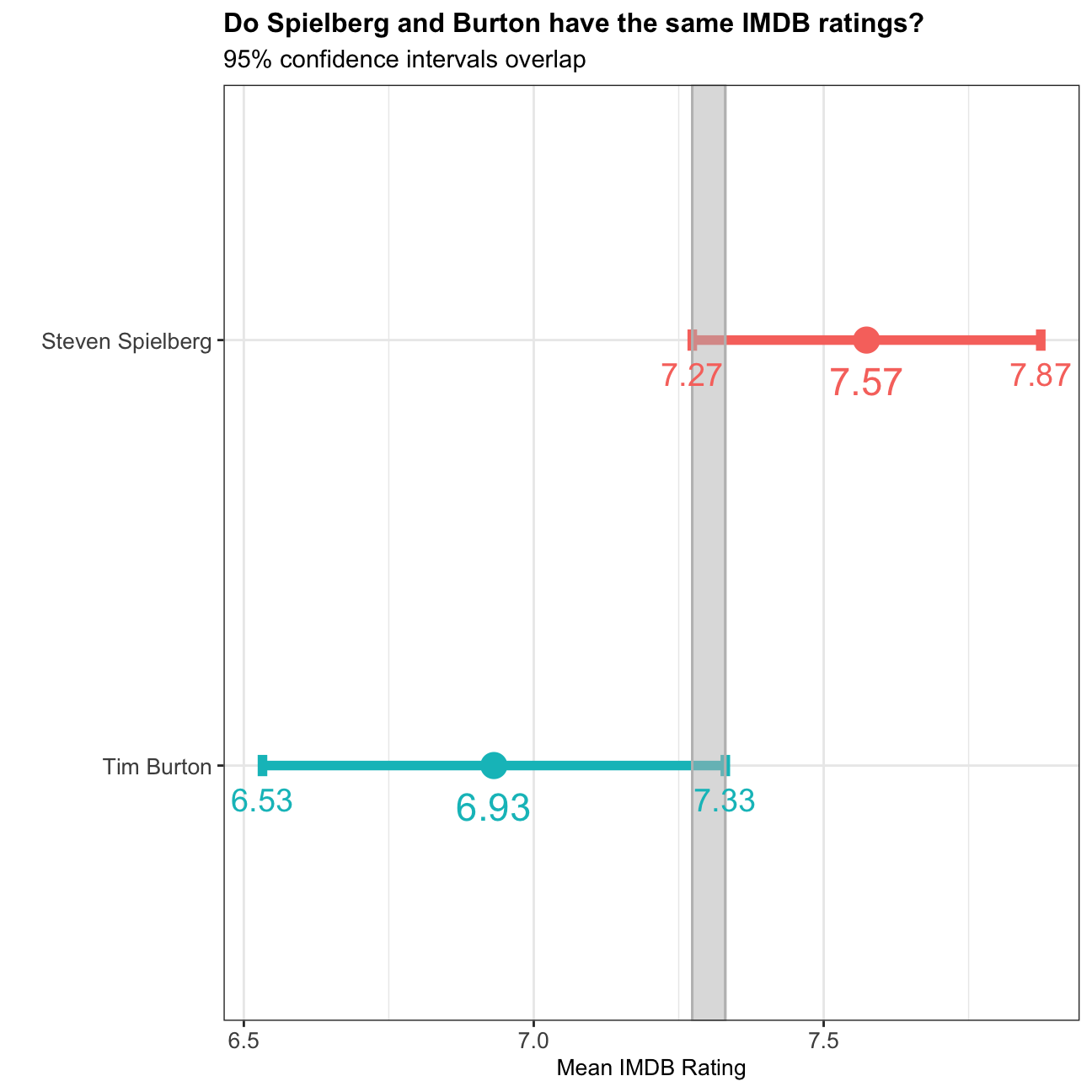

The overlap in 95% confidence intervals for the mean ratings means that we cannot yet say that movies of these two directors have different mean ratings.
Therefore, we need to conduct further tests to find out.

T-test command

First, we conduct a t-test using the existing sample and let’s see the summary statistics yielded by the t.test command.

#t-test command
S_B_ratings<- movies%>%
  filter(director %in% c("Steven Spielberg", "Tim Burton"))%>%
  select(director,rating)

  t.test(S_B_ratings$rating ~ S_B_ratings$director,
         mu=0,alt = "two.sided",conf=0.95,var.eq=FALSE)

## 
##  Welch Two Sample t-test
## 
## data:  S_B_ratings$rating by S_B_ratings$director
## t = 3, df = 31, p-value = 0.01
## alternative hypothesis: true difference in means is not equal to 0
## 95 percent confidence interval:
##  0.16 1.13
## sample estimates:
## mean in group Steven Spielberg       mean in group Tim Burton 
##                           7.57                           6.93

The t.test command result shows that the t-statistic is 2.7144, and the p-value is 0.01078, which are both indicators that the true difference in mean IMDB ratings between movies of Spielberg and Tim Burton is not zero. In addition, the 95% confidence interval also does not include zero.

Hypothesis Testing using ‘infer’ package

Other than doing a t-test, we can also arrive at our conclusion using hypothesis testing. In this case,

We then build a simulation using the infer package in and see if it supports our previous conclusion.

#t-test using "infer" package
null_ratings <- S_B_ratings %>%
  specify(rating ~ director) %>%
  hypothesize(null = "independence") %>%
  generate(reps = 1000, type = "permute") %>%
  calculate(stat = "diff in means", 
            order = c("Steven Spielberg", "Tim Burton"))

null_ratings%>%
  visualise()+
  labs(title = "Differences in Spielberg and Burton movie ratings in a world where there is really no difference",
       subtitle = "Observed difference in sample means marked in red", 
       x="Average ratings of Spielberg movies - Average ratings of Burton movies", 
       y = "Count")+
  theme_bw()+
  theme(plot.title = element_text(size = 15, face = "bold"),
        plot.subtitle = element_text(size = 10),
        axis.text = element_text(size = 10), 
        axis.title = element_text(size=10))+
  geom_rect(aes(xmin=0.64,xmax = Inf, ymin=-Inf,ymax=Inf),
            fill = "lightyellow", colour = "lightyellow", alpha=0.05)+
  geom_rect(aes(xmin=-Inf,xmax = -0.64, ymin=-Inf,ymax=Inf), 
            fill = "lightyellow", colour = "lightyellow", alpha=0.05)+
  geom_vline(aes(xintercept=0.64),colour = "red", size = 2)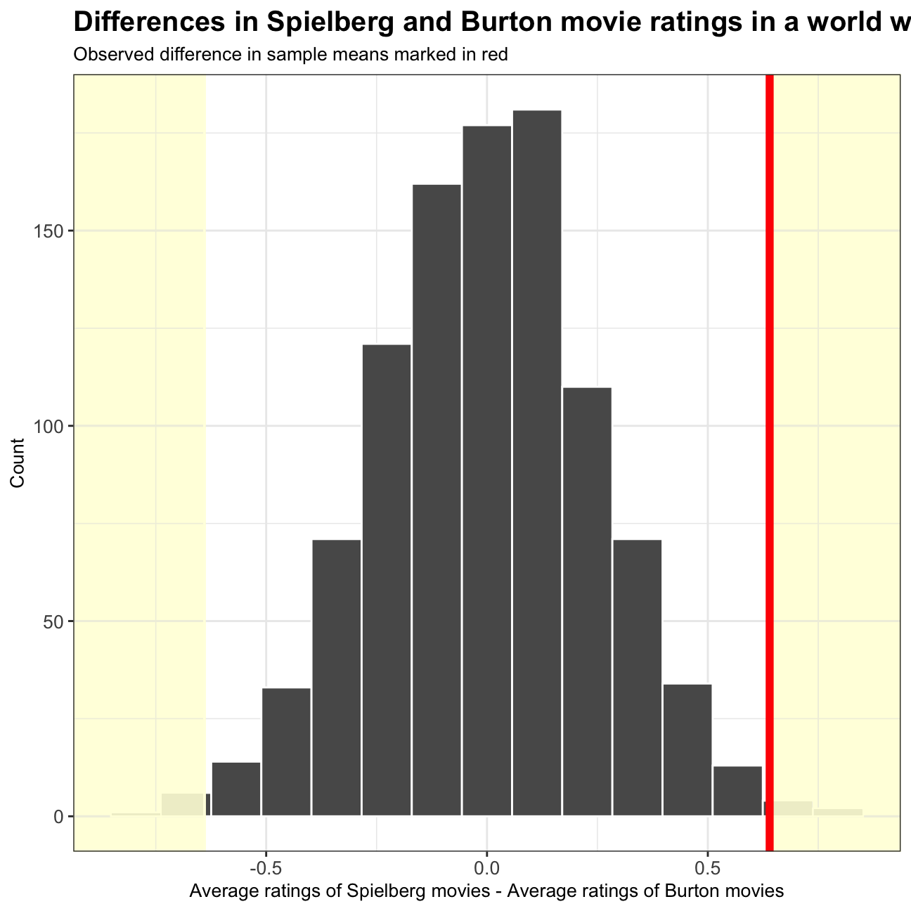

p_value <- null_ratings%>%
  get_pvalue(obs_stat = 0.64, direction = "both")

p_value

## # A tibble: 1 x 1
##   p_value
##     <dbl>
## 1   0.018

As we can see from the simulation results, the p-value is 0.01, which is also less than 0.05. Moreover, the graph also shows that the observed difference of mean movie ratings, as in our sample data, is 0.64. The number rather appears on the outer-right of this histogram, providing us with further evidence that we can reject the null hypothesis. That is, the true difference in mean IMDB ratings for movies directed by Steven Spielberg and Tim Burton, is different and therefore not zero.